The Ultimate Guide to Assessing Forest Cover and Land Eligibility for Forest Carbon Projects with Hansen and Dynamic World

Understanding an area's historical land cover, especially in forestation over the past decade, is crucial in the design of Nature-based Solutions. To aid in the complex task of assessing land eligibility, particularly for projects under the VM0047 (ARR) and VM0048 (REDD+) methodologies, Maya utilises two distinct datasets: The Global Forest Change dataset by Professor Matthew Hansen and Google’s Dynamic World.

This blog post explores these two datasets, highlighting their opportunities and limitations. We will delve into why there is no "one-size-fits-all" solution for assessing land cover for afforestation and conservation projects.

Check out our full analysis catalog to learn more about Maya’s analyses and integrated datasets from which you can benefit.

Content Overview

• Key Takeaways
• Hansen Global Forest Change
• Dynamic World
• Comparison: Hansen vs Dynamic World
• Eligible Area Analysis on Maya

‍Key Takeaways

1. Understand Dataset Strengths and Limitations: Be aware of each dataset’s specific constraints – such as Hansen’s lower resolution, annually available updates, and limited insights for your eligible area analysis due to a binary forest/non-forest classification. Dynamic World, on the other hand, is only been available since mid-2015, frequently experiences data gaps in cloudy regions and faces variability in the certainty behind land cover classifications due to its per-pixel probability method.

2. Customise Analysis Settings to Optimise Accuracy: Adjust the settings of the Hansen and Dynamic World datasets to accurately reflect the actual land cover. This includes modifying the canopy cover threshold in Hansen for a more accurate depiction of forest cover and tweaking class settings in Dynamic World for your eligible area analysis.

3. Leverage Comparative Analysis for Enhanced Decision Making: Compare the analysis outputs from Hansen and Dynamic World to identify discrepancies and validate accuracy. This comparative approach helps to determine which dataset provides the most reliable information for specific aspects of your project, aiding in more informed decision-making regarding land eligibility.

We’re here to support you in using and adjusting the most suitable dataset for your use cases, so let’s chat if that’s you!

Hansen Global Forest Change

The Hansen Global Forest Change dataset, developed by Professor Matthew Hansen and his team at the University of Maryland, is a crucial tool for assessing forest cover changes globally from 2000 onwards. Leveraging data from the Landsat satellite series, this dataset provides insights into forest dynamics and offers annual updates on tree cover and forest loss.

For limitations of this dataset regarding resolution, cloud cover issues, and underestimation of forest loss on smallholder land, please refer to our previous blog post, Maintaining a Clear View: The Most Commonly Used Geospatial Datasets for Assessing Nature-based Solutions.

How does Hansen define trees and forests in the dataset?

In their study and dataset, Hansen et al. define trees as all vegetation taller than 5m. They study tree cover extent, loss and gain based on a range of different canopy cover thresholds. For example, when using a threshold of 30% canopy density, a 30 x 30-meter pixel is classified as forest if the tree canopy cover is at least 30% of the pixel and classified as non-forest for all canopy cover below.

Which threshold is the best to use depends on the geographical location. Global Forest Watch (GFW), which uses Hansen for its Tree Canopy Cover dataset, follows a 30% canopy cover threshold in its definition but allows users to modify it to suit their purposes best. As most users know and trust the GFW dataset already, a 30% threshold is also the default setting on Maya.

Overall, these definitions are widely aligned with those of the Food and Agriculture Organization of the United Nations (FAO) and the United Nations Framework Convention on Climate Change (UNFCCC): FAO defines forest as “land spanning more than 0.5 hectares with trees higher than 5 meters and a canopy cover of more than 10%” (p. 4), and the UNFCCC as “a minimum area of land of 0.05-1.0 hectares with tree crown cover [...] of more than 10-30 per cent with trees with the potential to reach a minimum height of 2-5 metres” (p. 58).

‍Case Study I: Adjusting the Hansen Canopy Cover Threshold on Maya

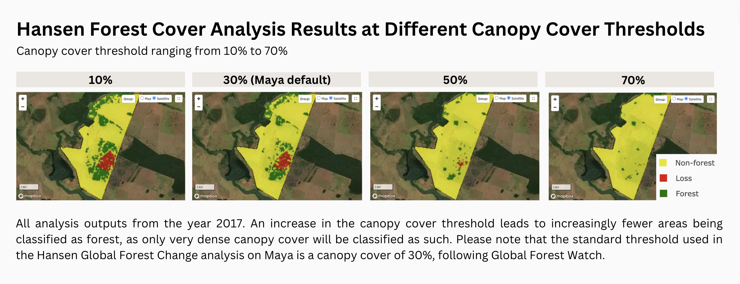
The output above shows fewer areas classified as forests as the canopy cover threshold increases. Lowering the Hansen dataset’s threshold (Maya default = 30%) is particularly useful in regions with generally sparse forest coverage, such as certain areas in Africa where the tree cover is naturally less dense. Setting a lower threshold allows a more accurate representation of these woodlands as forests. Changing the threshold in the analysis is a good tool for checking the robustness of the results.

Dynamic World 

The Dynamic World dataset is the result of a partnership between Google and the World Resources Institute to produce a dynamic dataset of the physical materials on the Earth’s surface. It offers a near real-time (updated every 2-5 days) land cover classification at a 10m resolution using a deep learning approach using Sentinel-2 imagery. It distinguishes between nine land use and cover classes: water, trees, grass, crops, shrub & scrub, flooded vegetation, built-up area, bare ground, and snow & ice.

How does Dynamic World classify trees in the dataset?

For their Dynamic World dataset, Brown et al. define trees as “any significant clustering of dense vegetation, typically with a closed or dense canopy” that is “taller and darker than surrounding vegetation (if surrounded by other vegetation)” (p. 3).

Unlike other traditional land cover datasets, this model does not use a specific threshold for tree classification. Instead, it provides a probability score for each of the 9 land cover classes, including trees, for every 10 x 10-meter pixel. For the “Trees” class, this is the estimated probability of complete coverage by trees, with values ranging between 0 and 1 (i.e., 0 to 100% probability). The class with the highest probability score is then assigned to that pixel. This approach allows for a more nuanced representation of land cover by considering the likelihood of each class rather than a binary classification based on a preset threshold​. However, as the final class allocation depends on the highest probability score, the certainty can vary: The highest probability score across all classes can be very high or can also be relatively low as long as it’s greater than the score of the other remaining classes.

Cloud coverage and training dataset implications

Cloud cover can significantly obstruct satellite imagery. This is a common issue in tropical regions, where much of the world’s forests are located and where cloud cover can be persistent, potentially leading to gaps in data or delays in detecting changes. When a satellite image has too many cloud pixels (>35%), Dynamic World typically excludes the whole image from the analysis.

Furthermore, the Dynamic World dataset’s reliance on a machine learning model means that its accuracy can vary depending on the training data and the representativeness of these data across all global conditions. Regions that are underrepresented in the training dataset or have less frequent satellite coverage due to persistent cloud cover can also experience higher classification errors.

Case Study II: Data Gaps and Misclassification

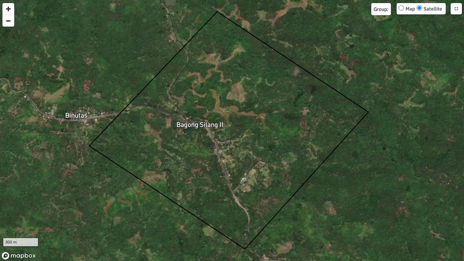
Let’s take this area of interest as an example. While most of it seems to be trees or forests, it is evident that there are buildings, roads, and what appears to be cropland or bare ground.

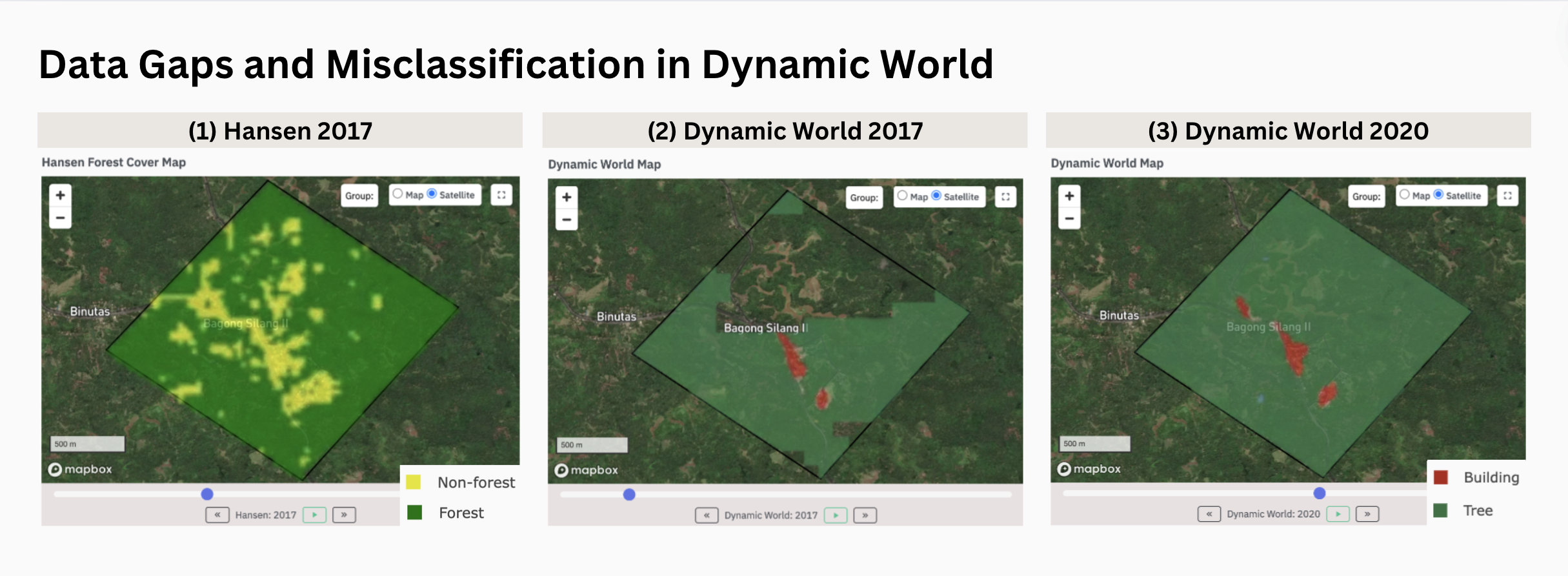
Looking at the geospatial analysis map outputs of Hansen (2017) and Dynamic World (2017 & 2020), one can see quite some differences in the classification of trees/forests: 

1. While we can’t say how correct Hansen is, we see that some areas have been correctly classified as non-forest along what we visually detected as buildings, roads, and cropland or bare land previously. The dataset seems to perform quite well. 
2. Dynamic World, on the other hand, has significant data gaps regarding its coverage of that specific area of interest in 2017. This is especially evident in areas that appear to be cropland or bare land. (Note: Maya depicts the yearly mode* of each pixel in the map.)
3. In 2020, the Dynamic World dataset has fewer data gaps, but it also classifies most of the area of interest as trees, apart from a few built-up areas. Comparing the result to the satellite image above, this seems to be a misclassification.

*The mode is the most frequently occurring value; in that case, the class assigned most often to a pixel over an analysed year.

Comparison: Hansen vs Dynamic World

Which dataset is best suited for my analysis?

Generally, it’s hard to say which dataset performs better, as this depends on regional characteristics and the specific objectives of the land cover analysis. Thus, understanding the strengths and limitations of each dataset in relation to the geographic and ecological context they are applied to is crucial for making informed decisions in assessing land cover for Nature-based Solutions.

At Maya, we want to ensure you have all the necessary tools to make informed decisions. It makes sense to test different Hansen canopy cover thresholds in regions with lots of cloud coverage, naturally sparse forests, or where Dynamic World doesn’t seem to perform very well. We know that making the right decisions in choosing and adjusting the right analysis job can be complicated, so please contact the Maya team. We are happy to discuss your cases together.

Eligible Area Analysis on Maya

Based on pre-defined rules, the VM0047 and VM0048 Eligible Area analyses select the area that was constantly (or was not at all) classified as trees or forest over the period analysed. 

For example, VM0047’s census-based approach requires that the “project activity must occur within an area classified as non-forest for the past ten years with less than 10% pre-existing woody biomass cover; and/or occur in an area subject to continuous cropping, in ‘settlements”, or “other lands’” (p. 9). The VM0047 eligible area analysis based on Hansen is now searching for areas that have been constantly classified as “non-forest” over the last 10 years prior to project start date. While doing so, the analysis allows for 0% historic tree/forest cover and does not consider the up to 10% allowed woody biomass, which can thus be regarded as conservative.

Eligible Area Selection Criteria

There are several adjustable selection criteria for Hansen and Dynamic World. For Hansen, you can adjust the canopy cover threshold to accommodate the needs of different geographic areas, as shown in Case Study I. You can also select a minimum plot size through which very small polygons smaller than, e.g., 0.5 hectares (Maya’s default) are excluded from the eligible area. 

For Dynamic World, choosing the right land cover types that you deem eligible for your project is especially important. For some areas of interest, you might want to deem Crops, Grass, Bare Land, and Shrubs/Scrubs as eligible for your ARR project, while for others, you might want to exclude Shrubs/Scrubs. Buildings and water will always be excluded from the eligible area, and you can decide how large the buffer around the two land cover types should be. The default setting on Maya includes a buffer of 10m (1 pixel) that is added around buildings and water bodies.

You can read more about the rule-based selection for the eligible area analyses in our Analysis Catalog:

• VM0047 Eligible Area (Hansen)
• VM0047 Eligible Area (Dynamic World)
• VM0048 Eligible Area (Hansen)
• VM0048 Eligible Area (Dynamic World)

‍Limitations of the Eligible Area Analysis

As with all geospatial analyses, the quality of the results will depend on the suitability of the dataset used within your specific area of interest, as shown in Case Study II. 

For the Eligible Area analysis, it is important to mention that Hansen only makes a binary differentiation between forest and non-forest. The non-forest category is a big cluster of all land cover and use types apart from forest, e.g., water, built-up areas, crops, grass, etc., and such a “black-and-white” classification with just two classes is typically associated with a better performance compared to having more classes. However, for the non-forest land cover check (VM0047 –  Eligible Area Analysis) this means that built-up areas like buildings or roads will also be included in the eligible area calculation, though they can not be afforested. 

When using the Dynamic World dataset for an eligibility analysis, it must be noted that the data is not available for the whole 10-year period of interest, as it is only available from mid-2015 onwards. While in some geographic areas, you might want to include Shrubs/Scrubs in your eligible area for an ARR project, you might want to exclude it in other projects. This is a decision you have to make for yourself, but we are happy to help you with that.

Case Study III: VM0047 Eligible Area Analysis based on Hansen and Dynamic World

In this exemplary potential ARR area of interest, Hansen classifies nearly 100% of the area as non-forest every year. Thus, the whole area is deemed eligible for an ARR project. Due to Hansen’s binary classification of forest and non-forest, the eligible area also includes parts that are definitely water and can thus not be afforested.

The Dynamic World dataset does a much more nuanced land cover analysis. It detects the permanent water resources, 20-40% tree cover, and lots of Shrubs/Scrubs. In this exemplary VM0047 Eligible Area analysis, the area classified as Shrubs/Scrubs, Crops, and Grass over the entire analysis period is deemed eligible after considering the buffer area and minimum plot size. Using the Dynamic World dataset, only about 50% of the area is detected as eligible for an ARR project.

If you’re still reading, you should be an expert in using the Hansen and Dynamic World dataset for land & forest cover and eligible area assessments by now. So, what are you waiting for? Request a free consultation on your geospatial analysis set up with one of our co-founders here and get started with your geospatial copilot.

Written by Delphine-Marie Zacharias 🧡